Google Cloud

1. What’s new with Google Cloud

   Want to know the latest from Google Cloud? Find it here in one handy location. Check back regularly for our newest updates, announcements, resources, events, learning opportunities, and more. 

   ---

   Tip: Not sure where to find what you’re looking for on the Google Cloud blog? Start here: Google Cloud blog 101: Full list of topics, links, and resources.

   ---

   May 5 - May 9

   • AI assisted development with MCP Toolbox for Databases
     We are excited to announce new updates to MCP Toolbox for Databases. Developers can now use Toolbox from their preferred IDE, such as Cursor, Windsurf, Claude Desktop, more and leverage our new pre-built tools such as execute_sql and list_tables for AI-assisted development with Cloud SQL for PostgreSQL, AlloyDB and self-managed PostgreSQL.
     • Get Started with MCP Toolbox for Databases

   Apr 28 - May 2

   • Itching to build AI agents? Join the Agent Development Kit Hackathon with Google Cloud! Use ADK to build multi-agent systems to solve challenges around complex processes, customer engagement, content creation, and more. Compete for over $50,000 in prizes and demonstrate the power of multi-agent systems with ADK and Google Cloud.
     • Submissions are open from May 12, 2025 to June 23, 2025.
     • Learn more and register here.

   Apr 21 - Apr 25

   • Iceland’s Magic: Reliving Solo Adventure through Gemini
     Embark on a journey through Iceland's stunning landscapes, as experienced on Gauti's Icelandic solo trip. From majestic waterfalls to the enchanting Northern Lights, Gautami then takes these cherished memories a step further, using Google's multi-modal AI, specifically Veo2, to bring static photos to life. Discover how technology can enhance and dynamically relive travel experiences, turning precious moments into immersive short videos. This innovative approach showcases the power of AI in preserving and enriching our memories from Gauti's unforgettable Icelandic travels. Read more.

   • Introducing ETLC - A Context-First Approach to Data Processing in the Generative AI Era: As organizations adopt generative AI, data pipelines often lack the dynamic context needed. This paper introduces ETLC (Extract, Transform, Load, Contextualize), adding semantic, relational, operational, environmental, and behavioral context. ETLC enables Dynamic Context Engines for context-aware RAG, AI co-pilots, and agentic systems. It works with standards like the Model Context Protocol (MCP) for effective context delivery, ensuring business-specific AI outputs. Read the full paper.

   Apr 14 - Apr 18

   • What’s new in Database Center
     With general availability, Database Center now provides enhanced performance and health monitoring for all Google Cloud databases, including Cloud SQL, AlloyDB, Spanner, Bigtable, Memorystore, and Firestore. It delivers richer metrics and actionable recommendations, helps you to optimize database performance and reliability, and customize your experience. Database Center also leverages Gemini to deliver assistive performance troubleshooting experience. Finally, you can track the weekly progress of your database inventory and health issues. 

     Get started with Database Center today

     • Access Database Center in Google Cloud console

     • Review the documentation to learn more

   Apr 7 - Apr 11

   • This week, at Google Cloud Next, we announced an expansion of Bigtable's SQL capabilities and introduced continuous materialized views. Bigtable SQL and continuous materialized views empower users to build fully-managed, real-time application backends using familiar SQL syntax, including specialized features that preserve Bigtable's flexible schema — a vital aspect of real-time applications. Read more in this blog.
   • DORA Report Goes Global: Now Available in 9 Languages!
     Unlock the power of DevOps insights with the DORA report, now available in 9 languages, including Chinese, French, Japanese, Korean, Portuguese, and Spanish. Global teams can now optimize their practices, benchmark performance, and gain localized insights to accelerate software delivery. The report highlights the significant impact of AI on software development, explores platform engineering’s promises and challenges, and emphasizes user-centricity and stable priorities for organizational success. Download the DORA Report Now
   • New Google Cloud State of AI Infrastructure Report Released
     Is your infrastructure ready for AI? The 2025 State of AI Infrastructure Report is here, packed with insights from 500+ global tech leaders. Discover the strategies and challenges shaping the future of AI and learn how to build a robust, secure, and cost-effective AI-ready cloud. Download the report and enhance your AI investments today. Download the 2025 AI infrastructure report now
   • Google Cloud and Oracle Accelerate Enterprise Modernization with New Regions, Expanded Capabilities
     Announcing major Oracle Database@Google Cloud enhancements! We're launching the flexible Oracle Base Database Service and powerful new Exadata X11M machines. We're rapidly expanding to 20 global locations, adding new Partner Cross-Cloud Interconnect options, and introducing Cross-Region Disaster Recovery for Autonomous Database. Benefit from enhanced Google Cloud Monitoring, integrated Backup & DR, plus expanded support for enterprise applications like SAP. Customers can run critical Oracle workloads with more power, resilience, and seamless Google Cloud integration. Get started right away from your Google Cloud Console or learn more here.

   Mar 17 - Mar 21

   • Cloud CISO Perspectives: 5 tips for secure AI success-To coincide with new AI Protection capabilities in Security Command Center, we’re offering 5 tips to set up your organization for secure AI success.
   • Our 4-6-3 rule for strengthening security ties to business:The desire to quickly transform a business can push leaders to neglect security and resilience, but prioritizing security can unlock value. Follow these 4 principles, 6 steps, and 3 metrics to use a security-first mindset to drive business results.
   • The new Data Protection Tab in Compute Engine ensures your resources are protected: Not only have we co-located your backup options, but we also have introduced smart default data protection for any Compute Engine instance created via Cloud Console. Here’s how it works.
   • DORA report - Impact of Generative AI in Software Development
     This report builds on and extends DORA's research into AI. We review the current landscape of AI adoption, look into its impact on developers and organizations, and outline a framework and practical guidance for successful integration, measurement, and continuous improvement. Download the report!

   Mar 10 - Mar 14

   • Protecting your APIs from OWASP’s top 10 security threats: We compare OWASP’s top 10 API security threats list to the security capabilities of Apigee. Here’s how we hold up.

   • Project Shield makes it easier to sign up, set up, automate DDoS protection: It’s now easier than ever for vulnerable organizations to apply to Project Shield, set up protection, and automate their defenses. Here’s how.

   • How Google Does It: Red teaming at Google scale- The best red teams are creative sparring partners for defenders, probing for weaknesses. Here’s how we do red teaming at Google scale.

   • AI Hypercomputer is a fully integrated supercomputing architecture for AI workloads – and it’s easier to use than you think. Check out this blog, where we break down four common use cases, including reference architectures and tutorials, representing just a few of the many ways you can use AI Hypercomputer today. 

   • Transform Business Operations with Gemini-Powered SMS-iT CRM on Google Cloud: SMS-iT CRM on Google Cloud unifies SMS, MMS, email, voice, and 22+ social channels into one Smart Inbox. Enjoy real-time voice interactions, AI chatbots, immersive video conferencing, AI tutors, AI operator, and unlimited AI agents for lead management. Benefit from revenue-driven automation, intelligent appointment scheduling with secure payments, dynamic marketing tools, robust analytics, and an integrated ERP suite that streamlines operations from project management to commerce. This comprehensive solution is designed to eliminate inefficiencies and drive exponential growth for your business.Experience the Future Today.

   • Join us for a new webinar,Smarter CX, Bigger Impact: Transforming Customer Experiences with Google AI, where we'll explore how Google AI can help you deliver exceptional customer experiences and drive business growth. You'll learn how to:

   • Transform Customer Experiences:  With conversational AI agents that provide personalized customer engagements.

   • Improve Employee Productivity & Experience: With AI that monitors customers sentiment in real-time, and assists customer service representatives to raise customer satisfaction scores.

   • Deliver Value Faster: With  30+ data connectors and 70+ action connectors to the most commonly used CRMs and information systems.
     
     Register here

   Mar 3 - Mar 7

   • Hej Sverige! Google Cloud launches new region in Sweden - More than just another region, it represents a significant investment in Sweden's future and Google’s ongoing commitment to empowering businesses and individuals with the power of the cloud. This new region, our 42nd globally and 13th in Europe, opens doors to opportunities for innovation, sustainability, and growth — within Sweden and across the globe. We're excited about the potential it holds for your digital transformations and AI aspirations.
   • [March 11th webinar] Building infrastructure for the Generative AI era: insights from the 2025 State of AI Infra report:Staying at the forefront of AI requires an infrastructure built for AI. Generative AI is revolutionizing industries, but it demands a new approach to infrastructure. In this webinar, we'll unveil insights from Google Cloud's latest research report and equip tech leaders with a practical roadmap for building and managing gen AI workloads, including: the top gen AI use cases driving the greatest return on investment, current infrastructure approaches and preferences for Generative AI workloads, the impact of performance benchmarks, scalability, and security on cloud provider selection. Register today.
   • Cloud CISO Perspectives: Why PQC is the next Y2K, and what you can do about it: Much like Y2K 25 years ago, post-quantum cryptography may seem like the future’s problem — but it will soon be ours if IT doesn’t move faster, explains Google Cloud’s Christiane Peters. Here's how business leaders can get going on PQC prep.
   • How Google Does It: Using threat intelligence to uncover and track cybercrime — How does Google use threat intelligence to uncover and track cybercrime? Google Threat Intelligence Group’s Kimberly Goody takes you behind the scenes.
   • 5 key cybersecurity strategies for manufacturing executives — Here are five key governance strategies that can help manufacturing executives build a robust cybersecurity posture and better mitigate the evolving risks they face.
   • Datastream now offers Salesforce source in Preview. Instantly connect, capture changes, and deliver data to BigQuery, Cloud Storage, etc. Power real-time insights with flexible authentication and robust backfill/CDC. Unlock Salesforce data for Google Cloud analytics, reporting, and generative AI. Read the documentation to learn more.
   • Find out how much you can save with Spanner -According to a recent Forrester Total Economic Impact™ study, by migrating to Spanner from a traditional database, a $1 billion per year B2C organization could get a 132% return on investment (ROI) with a 9-month payback period, and realize $7.74M in total benefits over the three years. To see how, check out the blog or download the report. 
   • GenAI Observability for Developers series: The Google Cloud DevRel team hosted a four-part webinar series, "Gen AI Observability for Developers," demonstrating observability best practices in four programming languages. Participants learned to instrument a sample application deployed on Cloud Run for auditing Vertex AI usage, writing structured logs, tracking performance metrics, and utilizing OpenTelemetry for tracing. The series covered Go, Java, NodeJS, and Python, using common logging and web frameworks. Missed it? Recordings and hands-on codelabs are available to guide you at:
     • Gen AI O11y for Go Developers
     • Gen AI O11y for Java Developers
     • Gen AI O11y for NodeJS Developers
     • Gen AI O11y for Python Developers
       
       Stay tuned for future events at cloudonair.withgoogle.com.

   Feb 24 - Feb 28

   • Rethinking 5G:Ericsson and Google Cloud are collaborating to redefine 5G mobile core networks with a focus on autonomous operations. By leveraging AI and cloud infrastructure, we aim to enhance efficiency, security, and innovation in the telecommunications industry. This partnership addresses the increasing demands of 5G and connected devices, paving the way for a more dynamic and intelligent network future, and setting the stage for next-generation technologies like 6G. Learn more here.
   • Adopt a principles-centered well-architected framework to design, build, deploy, and manage Google Cloud workloads that are secure, resilient, efficient, cost-efficient, and high-performing. Also get industry and technology-focused well-architected framework guidance, like for AI and ML workloads.

   Feb 17 - Feb 21

   • Easier Default Backup Configuration for Compute Engine Instances - The Create a Compute Instance page in the Google Cloud console now includes enhanced data protection options to streamline backup and replication configurations. By default, an option to back up data is pre-selected, ensuring recoverability in case of unforeseen events. Learn more here.

   Feb 10 - Feb 14

   • [Webinar] Generative AI for Software Delivery: Strategies for IT Leaders:Generative AI is transforming the way organizations build and deploy software. Join Google Cloud experts on February 26th to learn how organizations can leverage AI to streamline their software delivery, including: the role of gen AI in software development, how to use gen AI for migration and modernization, best practices for integrating gen AI into your existing workflows, and real-world applications of gen AI in software modernization and migration through live demos. Register here.

   Feb 3 - Feb 7

   • SQL is great but not perfect. We’d like to invite you to reimagine how you write SQL with Google’s newest invention: pipe syntax (public available to all BigQuery and Cloud Logging users). This new extension to GoogleSQL brings a modern, streamlined approach to data analysis. Now you can write simpler, shorter and more flexible queries for faster insights. Check out this video to learn more. 

   Jan 13 - Jan 17

   • C4A virtual machines with Titanium SSD—the first Axion-based, general-purpose instance with Titanium SSD,are now generally available. C4A virtual machines with Titanium SSDs are custom designed by Google for cloud workloads that require real-time data processing, with low-latency and high-throughput storage performance. Titanium SSDs enhance storage security and performance while offloading local storage processing to free up CPU resources. Learn more here.

   Jan 6 - Jan 10

   • A look back on a year of Earth Engine advancements:2024 was a landmark year for Google Earth Engine, marked by significant advancements in platform management, cloud integration, and core functionality and increased interoperability between Google Cloud tools and services. Here’s a round up of 2024’s top Earth Engine launches.
   • Get early access to our new Solar API data and features:We're excited to announce that we are working on 2 significant expansions to the Solar API from Google Maps Platform and are looking for trusted testers to help us bring them to market. These include improved and expanded buildings coverage and greater insights for existing solar installations with Detected Arrays. Learn more.
   • Google for Startups Accelerator: Women Founders applications are now open for women-led startups headquartered in Europe and Israel. Discover why this program could be the perfect fit for your startup and apply before January 24th, 2025.
   • Best of N: Generating High-Quality Grounded Answers with Multiple Drafts -We are excited to announce that Check Grounding API has released a new helpfulness score feature. Building on top of our existing groundedness score, we now enable users to implement Best of N to improve RAG response quality without requiring extensive model retraining. Learn more about Best of N and how it can help you here.

2. From LLMs to image generation: Accelerate inference workloads with AI Hypercomputer

   From retail to gaming, from code generation to customer care, an increasing number of organizations are running LLM-based applications, with78% of organizations in development or production today. As the number of generative AI applications and volume of users scale, the need for performant, scalable, and easy to use inference technologies is critical. At Google Cloud, we’re paving the way for this next phase of AI’s rapid evolution with our AI Hypercomputer. 

   At Google Cloud Next 25, we shared many updates toAI Hypercomputer’s inference capabilities, unveilingIronwood, our newest Tensor Processing Unit (TPU) designed specifically for inference, coupled with software enhancements such as simple and performant inference usingvLLM on TPU and the latestGKE inference capabilities —GKE Inference Gateway and GKE Inference Quickstart.

   With AI Hypercomputer, we also continue to push the envelope for performance with optimized software, backed by strong benchmarks: 

   • Google’sJetStream inference engine incorporates new performance optimizations, integrating Pathways for ultra-low latency multi-host, disaggregated serving.
   • MaxDiffusion, our reference implementation of latent diffusion models, delivers standout performance on TPUs for compute-heavy image generation workloads, and now supports Flux, one of the largest text-to-image generation models to date. 
   • The latest performance results fromMLPerf™ Inference v5.0 demonstrate the power and versatility of Google Cloud’s A3 Ultra (NVIDIA H200) and A4 (NVIDIA HGX B200) VMs for inference.

   Inference at scale with Google Cloud’s AI Hypercomputer

   Optimizing performance for JetStream: Google’s JAX inference engine

   To maximize performance and reduce inference costs, we are excited to offer more choice when serving LLMs on TPU, further enhancing JetStream and bringingvLLM support for TPU, a widely-adopted fast and efficient library for serving LLMs. With both vLLM on TPU andJetStream, we deliver standout price-performance with low-latency, high-throughput inference and community support through open-source contributions and from Google AI experts. 

   JetStream is Google’s open-source, throughput- and memory-optimized inference engine, purpose-built for TPUs and based on the same inference stack used to serve Gemini models.Since weannounced JetStream last April, we have invested significantly in further improving its performance across a wide range of open models. When using JetStream, our sixth-generation Trillium TPU now exceeds throughput performance by 2.9x for Llama 2 70B and 2.8x for Mixtral 8x7B compared to TPU v5e (using our reference implementationMaxText). 

   

   Available for the first time for Google Cloud customers, Google’sPathways runtime is now integrated into JetStream, enabling multi-host inference and disaggregated serving — two important features as model sizes grow exponentially and generative AI demands evolve.

   Multi-host inference using Pathways distributes the model across multiple accelerators hosts when serving. This enables the inference of large models that don't fit on a single host. With multi-host inference, JetStream achieves 1703 token/s on Llama 3.1 405B on Trillium. This translates to three times more inference per dollar compared to TPU v5e.

   In addition, with Pathways,disaggregated serving capabilities allow workloads to dynamically scale LLM inference’s decode and prefill stages independently. This allows for better utilization of resources and can lead to improvements in performance and efficiency, especially for large models. For Llama2-70B, using multiple hosts with disaggregated serving performs seven times better for prefill (time-to-first-token, TTFT) operations, and nearly three times better for token generation (time-per-output-token, TPOT) compared with interleaving the prefill and decode stages of LLM request processing on the same server on Trillium.

   

   

   Customers likeOsmos are using TPUs to maximize cost-efficiency for inference at scale:

   “Osmos is building the world's first AI Data Engineer. This requires us to deploy AI technologies at the cutting edge of what is possible today. We are excited to continue our journey  building on Google TPUs as our AI infrastructure for training and inference. We have vLLM and JetStream in scaled production deployment on Trillium and are able to achieve industry leading performance at over 3500 tokens/sec per v6e node for long sequence inference for 70B class models. This gives us industry leading tokens/sec/$, comparable to not just other hardware infrastructure, but also fully managed inference services. The availability of TPUs and the ease of deployment on AI Hypercomputer lets us build out an Enterprise software offering with confidence.”- Kirat Pandya, CEO, Osmos

   MaxDiffusion: High-performance diffusion model inference

   Beyond LLMs, Trillium demonstrates standout performance on compute-heavy workloads like image generation.MaxDiffusion delivers a collection of reference implementations of various latent diffusion models. In addition to Stable Diffusion inference, we have expanded MaxDiffusion to now support Flux; with 12 billion parameters, Flux is one of the largest open source text-to-image models to date. 

   As demonstrated on MLPerf 5.0, Trillium now delivers 3.5x throughput improvement for queries/second on Stable Diffusion XL (SDXL) compared to last performance round for its predecessor, TPU v5e. This further improves throughput by 12% since the MLPerf 4.1 submission.

   

   With this throughput, MaxDiffusion delivers a cost-efficient solution. The cost to generate 1000 images is as low as 22 cents on Trillium, 35% less compared to TPU v5e. 

   

   A3 Ultra and A4 VMs MLPerf 5.0 Inference results

   ForMLPerf™ Inference v5.0, we submitted 15 results, including our first submission with A3 Ultra (NVIDIA H200) andA4 (NVIDIA HGX B200) VMs. The A3 Ultra VM is powered by eight NVIDIA H200 Tensor Core GPUs and offers 3.2 Tbps of GPU-to-GPU non-blocking network bandwidth and twice the high bandwidth memory (HBM) compared to A3 Mega with NVIDIA H100 GPUs. Google Cloud's A3 Ultra demonstrated highly competitive performance, achieving results comparable to NVIDIA's peak GPU submissions across LLMs, MoE, image, and recommendation models. 

   Google Cloud was the only cloud provider to submit results on NVIDIA HGX B200 GPUs, demonstrating excellent performance of A4 VM for serving LLMs including Llama 3.1 405B (a new benchmark introduced in MLPerf 5.0). A3 Ultra and A4 VMs both deliver powerful inference performance, a testament to our deep partnership with NVIDIA to provide infrastructure for the most demanding AI workloads.

   Customers likeJetBrains are using Google Cloud GPU instances to accelerate their inference workloads:

   “We’ve been using A3 Mega VMs with NVIDIA H100 Tensor Core GPUs on Google Cloud to run LLM inference across multiple regions. Now, we’re excited to start using A4 VMs powered by NVIDIA HGX B200 GPUs, which we expect will further reduce latency and enhance the responsiveness of AI in JetBrains IDEs.”- Vladislav Tankov, Director of AI, JetBrains

   AI Hypercomputer is powering the age of AI inference

   Google's innovations in AI inference, including hardware advancements in Google Cloud TPUs and NVIDIA GPUs, plus software innovations such as JetStream, MaxText, and MaxDiffusion, are enabling AI breakthroughs with integrated software frameworks and hardware accelerators. Learn more about usingAI Hypercomputer for inference. Then, check out theseJetStream andMaxDiffusion recipes to get started today.

3. Expanding BigQuery geospatial capabilities with Earth Engine raster analytics

   At Google Cloud Next 25, we announced a major step forward in geospatial analytics:Earth Engine in BigQuery. This new capability unlocksEarth Engine raster analytics directly in BigQuery, making advanced analysis of geospatial datasets derived from satellite imagery accessible to the SQL community.

   Before we get into the details of this new capability and how it can power your use cases, it's helpful to distinguish between two types of geospatial data and where Earth Engine and BigQuery have historically excelled: 

   • Raster data: This type of data represents geographic information as a grid of cells, or pixels, where each pixel stores a value that represents a specific attribute such as elevation, temperature, or land cover. Satellite imagery is a prime example of raster data. Earth Engine excels at storing and processing raster data, enabling complex image analysis and manipulation.

   • Vector data: This type of data represents geographic features such as points, lines, or polygons. Vector data is ideal for representing discrete objects like buildings, roads, or administrative boundaries. BigQuery is highly efficient at storing and querying vector data, making it well-suited for large-scale geographic analysis.

   Earth Engine and BigQuery are both powerful platforms in their own right. By combining their geospatial capabilities, we are bringing the best of both raster and vector analytics to one place. That’s why we createdEarth Engine in BigQuery, an extension to BigQuery's current geospatial capabilities that will broaden access to raster analytics and make it easier than ever before to answer a wide range of real-world enterprise problems. 

   Earth Engine in BigQuery: Key features

   You can use the two key features of Earth Engine in BigQuery to perform raster analytics in BigQuery:

   • A new function in BigQuery: RunST_RegionStats(), anew BigQuery geography function that lets you efficiently extract statistics from raster data within specified geographic boundaries.

   • New Earth Engine datasets in BigQuery Sharing (formerly Analytics Hub): Access a growing collection of Earth Engine datasets inBigQuery Sharing (formerly Analytics Hub), simplifying data discovery and access. Many of these datasets areanalysis-ready, immediately usable for deriving statistics for an area of interest, and providing valuable information such as elevation, emissions, or risk prediction. 

   Five easy steps to raster analytics

   The newST_RegionStats() function is similar to Earth Engine’sreduceRegion function, which allows you to compute statistics for one or more regions of an image. TheST_RegionStats() function is a new addition toBigQuery’s set of geography functions invoked as part of any BigQuery SQL expression. It takes an area of interest (e.g., a county, parcel of land, or zip code) indicated by a geography and an Earth Engine-accessible raster image and computes a set of aggregate values for the pixels that intersect with the specified geography. Examples of aggregate statistics for an area of interest would be maximum flood depth or average methane emissions for a certain county. 

   These are the five steps to developing meaningful insights for an area of interest:

   1. Identify a BigQuery table with vector data: This could be data representing administrative boundaries (e.g., counties, states), customer locations, or any other geographic areas of interest. You can pull a dataset fromBigQuery public datasets or use your own based on your needs.

   2. Identify a raster dataset: You can discover Earth Engine raster datasets inBigQuery Sharing, or you can use raster data stored as aCloud GeoTiff orEarth Engine image asset. This can be any raster dataset that contains the information you want to analyze within the vector boundaries.

   3. UseST_RegionStats() to bring raster data into BigQuery: TheST_RegionStats() geography function takes the raster data (raster_id), vector geometries (geography), and optional band (band_name) as inputs and calculates aggregate values (e.g., mean, min, max, sum, count) on the intersecting raster data and vector feature. 

   4. Analyze the results: You can use the output of runningST_RegionStats() to analyze the relationship between the raster data and the vector features, generating valuable insights about an area of interest.

   5. Visualize the results: Geospatial analysis is usually most impactful when visualized on a map. Tools likeBigQuery Geo Viz allow you to easily create interactive maps that display your analysis results, making it easier to understand spatial patterns and communicate findings.

   Toward data-driven decision making

   The availability ofEarth Engine in BigQuery opens up new possibilities for scaled data-driven decision-making across various geospatial and sustainability use cases, by enabling raster analytics on datasets that were previously unavailable in BigQuery. These datasets can be used with the newST_RegionStats() geography function for a variety of use cases, such as calculating different land cover types within specific administrative boundaries or analyzing the average elevation suitability within proposed development areas. You can also find sample queries for these datasets in BigQuery Sharing’s individual dataset pages. For example, if you navigate to theGRIDMET CONUS Drought Indices dataset page, you can find asample query for calculating mean Palmer Drought Severity Index (PDSI) for each county in California, used to monitor drought conditions across the United States.

   Let’s take a deeper look at some of the use cases that this new capability unlocks:

   1. Climate, physical risk, and disaster response

   Raster data can provide critical insights on weather patterns and natural disaster monitoring. Many of the raster datasets available in BigQuery Sharing provide derived data on flood mapping, wildfire risk assessment, drought conditions, and more. These insights can be used for disaster risk and response, urban planning, infrastructure development, transportation management, and more. For example, you could use theWildfire Risk to Communities dataset for predictive analytics, allowing you to assess wildfire hazard risk, exposure of communities, and vulnerability factors, so you can develop effective resilience strategies. For flood mapping, you could use theGlobal River Flood Hazard dataset to understandregions in the US that have the highest predicted inundation depth, or water height above ground surface.

   2. Sustainable sourcing and agriculture 

   Raster data also provides insights on land cover and land use over time. Several of the new Earth Engine datasets in BigQuery include derived data on terrain, elevation, and land-cover classification, which are critical inputs for supply chain management and assessing agriculture and food security. For businesses that operate in global markets, sustainable sourcing requires bringing transparency and visibility to supply chains, particularly as regulatory requirements are shifting commitments todeforestation-free commodity production from being voluntary to mandatory. With the newForest Data Partnership maps for cocoa, palm and rubber, you can analyze where commodities are grown over time, and add in theForest Persistence or theJRC Global Forest Cover datasets to understand if those commodities are being grown in areas that had not been deforested or degraded before 2020. With a simple SQL query, you could, for instance,determine the estimated fraction of Indonesia's land area that had undisturbed forest in 2020.  

   3. Methane emissions monitoring 

   Reducing methane emissions from the oil and gas industry is crucial to slow the rate of climate change. TheMethaneSAT L4 Area Sources dataset, which can be used asan Earth Engine Image asset with the ST_RegionStats() function, provides insights into small, dispersed area emissions of methane from various sources. This type of diffuse but widespread emissions can make up the majority of methane emissions in an oil and gas basin. You can analyze the location, magnitude, and trends of these emissions to identify hotspots, inform mitigation efforts, and understand how emissions are characterized across large areas, such as basins. 

   4. Custom use cases

   In addition to these datasets, you can bring your own raster datasets viaCloud Storage GeoTiffs orEarth Engine image assets, to support other use cases, while still benefiting from BigQuery's scalability and analytical tools.

   aside_block

   <ListValue: [StructValue([('title', '$300 in free credit to try Google Cloud data analytics'), ('body', <wagtail.rich_text.RichText object at 0x3ef3802e8880>), ('btn_text', 'Start building for free'), ('href', 'http://console.cloud.google.com/freetrial?redirectPath=/bigquery/'), ('image', None)])]>

   Bringing it all together with an example 

   Let’s take a look at a more advanced example based on modeled wildfire risk and AI-driven weather forecasting technology. The SQL below uses theWildfire Risk to Communities dataset listed in BigQuery Sharing, which is designed to help communities understand and mitigate their exposure to wildfire. The data contains bands that index the likelihood and consequence of wildfire across the landscape. Using geometries from a public dataset of census-designated places, you can compute values from this dataset usingST_RegionStats() to compare communities’ relative risk exposures. You can also combine weather data fromWeatherNext Graph forecasts to see how imminent fire weather is predicted to affect those communities. 

   To start, head to theBigQuery Sharing console, click “Search listings”, filter to “Climate and environment,” select the “Wildfire Risk to Community” dataset (or search for the dataset in the search bar), and click “Subscribe” to add theWildfire Risk dataset to your BigQuery project. Then search for “WeatherNext Graph” and subscribe to theWeatherNext Graph dataset.

   

   With these subscriptions in place, run a query to combine these datasets across many communities with a single query. You can break this task into subqueries using the SQLWITH statement for clarity:

   First, select the input tables that you subscribed to in the previous step.

   Second, compute the weather forecast using WeatherNext Graph forecast data for a specific date and for the places of interest. The result is the average and maximum wind speeds within each community. 

   Third, use theST_RegionStats() function to sample the Wildfire Risk to Community raster data for each community. Since we are only concerned with computing mean values within regions, you can set the scale to 1 kilometer in the function options in order to use lower-resolution overviews and thus reduce compute time. To compute at the full resolution of the raster (in this case, 30 meters), you can leave this option out. 

   WITH
    -- Step 1: Select inputs from datasets that we've subscribed to
    wildfire_raster AS (
      SELECT
        id
      FROM
        `wildfire_risk_to_community_v0_mosaic.fire`
    ),
    places AS (
      SELECT
        place_id,
        place_name,
        place_geom AS geo,
      FROM
        `bigquery-public-data.geo_us_census_places.places_colorado`
    ),
   
   
    -- Step 2: Compute the weather forecast using WeatherNext Graph forecast data
    weather_forecast AS (
      SELECT
        ANY_VALUE(place_name) AS place_name,
        ANY_VALUE(geo) AS geo,
        AVG(SQRT(POW(t2.`10m_u_component_of_wind`, 2)
                 + POW(t2.`10m_v_component_of_wind`, 2))) AS average_wind_speed,
        MAX(SQRT(POW(t2.`10m_u_component_of_wind`, 2)
                 + POW(t2.`10m_v_component_of_wind`, 2))) AS maximum_wind_speed
      FROM
        `weathernext_graph_forecasts.59572747_4_0` AS t1,
        t1.forecast AS t2
      JOIN
        places
      ON
        ST_INTERSECTS(t1.geography_polygon, geo)
      WHERE
        t1.init_time = TIMESTAMP('2025-04-28 00:00:00 UTC')
        AND t2.hours < 24
      GROUP BY
        place_id
    ),
   
   
    -- Step 3: Combine with wildfire risk for each community
    wildfire_risk AS (
      SELECT
        geo,
        place_name,
        ST_REGIONSTATS(                      -- Wildfire likelihood
          geo,                               -- Place geometry
          (SELECT id FROM wildfire_raster),  -- Raster ID
          'RPS',                             -- Band name (Risk to Potential Structures)
          OPTIONS => JSON '{"scale": 1000}'  -- Computation resolution in meters
        ).mean AS wildfire_likelihood,
        ST_REGIONSTATS(                      -- Wildfire consequence
          geo,                               -- Place geometry
          (SELECT id FROM wildfire_raster),  -- Raster ID
          'CRPS',                            -- Band name (Conditional Risk to Potential Structures)
          OPTIONS => JSON '{"scale": 1000}'  -- Computation resolution in meters
        ).mean AS wildfire_consequence,
        weather_forecast.* EXCEPT (geo, place_name)
      FROM
        weather_forecast
    )
   
   
    -- Step 4: Compute a composite index of relative wildfire risk.
   SELECT
     *,
     PERCENT_RANK() OVER (ORDER BY wildfire_likelihood)
       * PERCENT_RANK() OVER (ORDER BY wildfire_consequence)
       * PERCENT_RANK() OVER (ORDER BY average_wind_speed)
       AS relative_risk
   FROM
     wildfire_risk

   The result is a table containing the mean values of wildfire risk for both bands within each community and wind speeds projected over the course of a day. In addition, you can combine the computed values for wildfire risk, wildfire consequence, and maximum wind speed into a single composite index to show relative wildfire exposure for a selected day in Colorado.

   

   You can save this output in Google Sheets to visualize how wildfire risk and consequences are related among communities statewide.

   

   Alternatively, you can visualize relative wildfire risk exposure inBigQuery GeoViz with the single composite index to show relative wildfire exposure for a selected day in Colorado.

   

   What’s next for Earth Engine in BigQuery?

   Earth Engine in BigQuery marks a significant advancement in geospatial analytics, and we’re excited to further expand raster analytics in BigQuery, making sustainability decision-making easier than ever before. Learn more about this new capability in theBigQuery documentation for working with raster data, and stay tuned for new Earth Engine capabilities in BigQuery in the near future!

4. New column-granularity indexing in BigQuery offers a leap in query performance

   BigQuery deliversoptimized search/lookup query performance by efficiently pruning irrelevant files. However, in some cases, additional column information is required for search indexes to further optimize query performance. To help, werecently announced indexing with column granularity, which lets BigQuery pinpoint relevant data within columns, for faster search queries and lower costs. 

   BigQuery arranges table data into one or more physical files, each holding N rows. This data is stored in a columnar format, meaning each column has its own dedicated file block. You can learn more about this in theBigQuery Storage Internals blog. The default search index is at the file level, which means it maintains mappings from a data token to all the files containing it. Thus, at query time, the search index helps reduce the search space by only scanning those relevant files. This file-level indexing approach excels when search tokens are selective, appearing in only a few files. However, scenarios arise where search tokens are selective within specific columns but common across others, causing these tokens to appear in most files, and thus diminishing the effectiveness of file-level indexes.

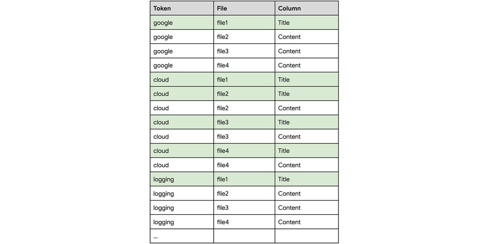
   For example, imagine a scenario where we have a collection of technical articles stored in a simplified table namedTechArticles with two columns —TitleandContent. And let's assume that the data is distributed across four files, as shown below.

   

   Our goal is to search for articles specifically related to Google Cloud Logging. Note that:

   • The tokens "google", "cloud", and "logging" appear in every file.

   • Those three tokens  also appear in the "Title" column, but only in the first file.

   • Therefore, the combination of the three tokens is common overall, but highly selective in the "Title" column.

   Now, let’s say, wecreate a search index on both columns of the table with the following DDL statement:

   CREATE SEARCH INDEX myIndex ON myDataset.TechArticles(Title, Content);

   The search index stores the mapping of data tokens to the data files containing the tokens, without any column information; the index looks like the following (showing the three tokens of interest: "google", "cloud", and "logging"):

   

   With the usual querySELECT * FROM TechArticles WHERE SEARCH(Title, "Google Cloud Logging"), using the index without column information, BigQuery ends up scanning all four files, adding unnecessary processing and latency to your query.

   aside_block

   <ListValue: [StructValue([('title', '$300 in free credit to try Google Cloud data analytics'), ('body', <wagtail.rich_text.RichText object at 0x3ef380797700>), ('btn_text', 'Start building for free'), ('href', 'http://console.cloud.google.com/freetrial?redirectPath=/bigquery/'), ('image', None)])]>

   Indexing with column granularity

   Indexing with column granularity, a new public preview feature in BigQuery, addresses this challenge by adding column information in the indexes. This lets BigQuery leverage the indexes to pinpoint relevant data within columns, even when the search tokens are prevalent across the table's files.

   Let’s go back to the above example. Now we can create the index with COLUMN granularity as follows:

   CREATE SEARCH INDEX myIndex ON myDataset.TechArticles(Title, Content)
   OPTIONS (default_index_column_granularity = 'COLUMN');

   The index now stores the column information associated with each data token. The index is as follows:

   

   Using the same querySELECT * FROM TechArticles WHERE SEARCH(Title, "Google Cloud Logging") as above but using the index with column information, BigQuery now only needs to scanfile1 since the index lookup is the intersection of the following:

   • Files where Token='google' AND Column='Title' (file1)

   • Files where Token='cloud' AND Column='Title' (file1, file2, file3, and file4)

   • Files where Token'='logging' AND Column='Title' (file1).

   Performance improvement benchmark results

   We benchmarked query performance on a 1TB table containingGoogle Cloud Logging data of an internal Google test project with the following query:

   SELECT COUNT(*)
   FROM `dataset.log_1T`
   WHERE SEARCH((logName, trace, labels, metadata), 'appengine');

   In this benchmark query, the token 'appengine' appears infrequently in the columns used for query filtering, but is more common in other columns. The default search index already helped reduce a large portion of the search space, resulting in half the execution time, reducing processed bytes and slot usage. By employing column granularity indexing, the improvements are even more significant.

   

   In short, column-granularity indexing in BigQuery offers the following benefits: 

   • Enhanced query performance: By precisely identifying relevant data within columns, column-granularity indexing significantly accelerates query execution, especially for queries with selective search tokens within specific columns.

   • Improved cost efficiency: Index pruning results in reduced bytes processed and/or slot time, translating to improved cost efficiency.

   This is particularly valuable in scenarios where search tokens are selective within specific columns but common across others, or where queries frequently filter or aggregate data based on specific columns.

   Best practices and getting started

   Indexing with column granularity represents a significant advancement in BigQuery's indexing capabilities, letting you achieve greater query performance and cost efficiency.

   For best results, consider the following best practices:

   • Identify high-impact columns: Analyze your query patterns to identify columns that are frequently used in filters or aggregations and would benefit from column-granularity indexing.

   • Monitor performance: Continuously monitor query performance and adjust your indexing strategy as needed.

   • Consider indexing and storage costs: While column-granularity indexing can optimize query performance, be mindful of potential increases in indexing and storage costs.

   To get started, simply enable indexing with column granularity. For more information, refer to theCREATE SEARCH INDEX DDL documentation.

5. How Looker’s semantic layer enables trusted AI for business intelligence

   In the AI era, where data fuels intelligent applications and drives business decisions, demand for accurate and consistent data insights has never been higher. However, the complexity and sheer volume of data coupled with the diversity of tools and teams can lead to misunderstandings and inaccuracies. That's why trusted definitions managed by a semantic layer become indispensable. Armed with unique information about your business, with standardized references, the semantic layer provides a business-friendly and consistent interpretation of your data, so that your AI initiatives and analytical endeavors are built on a foundation of truth and can drive reliable outcomes.

   Looker’s semantic layer acts as a single source of truth for business metrics and dimensions, helping to ensure that your organization and tools are leveraging consistent and well-defined terms. By doing so, the semantic layer offers a foundation for generative AI tools to interpret business logic, not simply raw data, meaning answers are accurate, thanks to critical signals that map to business language and user intent, reducing ambiguity. LookML (Looker Modeling Language) helps you create the semantic model that empowers your organization to define the structure of your data and its logic, and abstracts complexity, easily connecting your users to the information they need.

   A semantic layer is particularly important in the context of gen AI. When applied directly to ungoverned data, gen AI can produce impressive, but fundamentally inaccurate and inconsistent results. It sometimes miscalculates important variables, improperly groups data, or misinterprets definitions, including when writing complex SQL. The result can be misguided strategy and missed revenue opportunities. 

   In any data-driven organization, trustworthy business information is non-negotiable. Our own internal testing has shown that Looker’s semantic layer reduces data errors in gen AI natural language queries by as much as two thirds.According to a recent report by Enterprise Strategy Group, ensuring data quality and consistency proved to be the top challenge for organizations’ analytics and business intelligence platform. Looker provides a single source of truth, ensuring data accuracy and delivering trusted business logic for the entire organization and all connected applications.

   aside_block

   <ListValue: [StructValue([('title', 'Try Google Cloud for free'), ('body', <wagtail.rich_text.RichText object at 0x3ef3849d9fd0>), ('btn_text', 'Get started for free'), ('href', 'https://console.cloud.google.com/freetrial?redirectPath=/welcome'), ('image', None)])]>

   The foundation of trustworthy Gen AI

   To truly trust gen AI, it needs to be anchored to a robust semantic layer, which acts as your organization's data intelligence engine, providing a centralized, governed framework that defines your core business concepts and helping to ensure a single, consistent source of truth.

   The semantic layer is essential to deliver on the promise of trustworthy gen AI for BI, offering:

   • Trust: Reduce gen AI "hallucinations" by grounding AI responses in governed, consistently defined data. 

   • Deep business context: AI and data agents should know your business as well as your analysts do. You can empower those agents with an understanding of your business language, metrics, and relationships to accurately interpret user queries and deliver relevant answers.

   • Governance: Enforce your existing data security and compliance policies within the gen AI environment, protecting sensitive information and providing auditable data access.

   • Organizational alignment: Deliver data consistency across your entire organization, so every user, report and AI-driven insight are using the same definitions and terms and referring to them the same way.

   

   The semantic layer advantage in the gen AI era

   LookML, Looker’s semantic modeling language, is architected for the cloud and offers a number of critical values for fully integrating gen AI in BI:

   • Centralized definitions: Experts can define metrics, dimensions, and join relationships once, to be re-used across all Looker Agents, chats and users, ensuring consistent answers that get everyone on the same page.

   • Deterministic advanced calculations: Ideal for complex mathematical or logistical operations, Looker eliminates randomness and provides predictable and repeatable outcomes. Additionally, our dimensionalized measures capability aggregates values so you can perform operations on them as a group, letting you perform complex actions quickly and simply.

   • Software engineering best practices: With continuous integration and version control, Looker ensures code changes are frequently tested and tracked, keeping production applications running smoothly.

   • Time-based analysis: Built-in dimension groups allow for time-based and duration-based calculations.

   • Deeper data drills: Drill fields allow users to explore data in detail through exploration of a single data point. Data agents can tap into this capability and assist users to dive deeper into different slices of data.

   With the foundation of a semantic layer, rather than asking an LLM to write SQL code against raw tables with ambiguous field names (e.g.,order.sales_sku_price_US), the LLM is empowered to do what it excels at: searching through clearly defined business objects within LookML (e.g.,Orders > Total Revenue). These objects can include metadata and human-friendly descriptions (e.g., "The sum of transaction amounts or total sales price"). This is critical when business users speak in the language of business — “show me revenue” — versus the language of data — ”show me sum of sales (price), not quantity.” LookML bridges the data source and what a decision-maker cares about, so an LLM can better identify the correct fields, filters, and sorts and turn data agents into intelligent ad-hoc analysts.

   LookML offers you a well-structured library catalog for your data, enabling an AI agent to find relevant information and summaries, so it can accurately answer your question. Looker then handles the task of actually retrieving that information from the right place.

   The coming together of AI and BI promises intelligent, trustworthy and conversational insights. Looker's semantic layer empowers our customers to gain benefit from these innovations in all the surfaces where they engage with their data. We will continue to expand support for a wide variety of data sources, enrich agent intelligence, and add functionality to conversational analytics to make data interaction as intuitive and powerful as a conversation with your most trusted business advisor.

   To gain the full benefits of Looker’s semantic layer and Conversation Analytics, get startedhere. To learn more about the Conversational Analytics API, see our recent update from Google Cloud Next, orsign up here for preview access.